
Use this sigma calculator to very quickly figure out process sigma levels, DPMO / PPM, yield, rolled throughput yield, percentage of defects, units with defects, and defects per million units. You are able to type in the number set combinations of data; however, for the most pertinent information, just give defects, units, and defect opportunities per unit respective amounts. The calculator can also tell you how many samples you need to keep process yield at a certain level per standard.
Using the Sigma Level Calculator
This Sigma Calculator will help you get the sigma level of your process (the output is the defect rate you produce in units or deliver as a service). The output is dependent upon the input and may vary
- process sigma (comparative quality but how tight its control is to the acceptance standard)
- regard ranges as opportunities missed from an actual defect (standard yield)
- acceptable products or services delivered (rolled throughput yield: RTY) in terms of yield
- percentage DPMO (defects million opportunities, aka ppm)
- defect units out of total production
- Defects per million units (DPM)
If DPMO is the least required input, the Six Sigma calculator (which is not a notation sigma converter! ) tells you the correct sigma level, yield, and percent defect. Upon entering the number of defects and total opportunities for defects to happen, the control level (sigma), yield percent defect, etc., are calculated. With this tool being entered by defects, units, and opportunities per unit (number of specifications that have to be within quality for every unit, defect opportunity per unit) will result in the total output of the calculator, i.e., DPM included percentage of defective units and RTY together along with already mentioned covered outputs.
What is Six Sigma in process control?
Quality of industrial control in production quality and broadly project management (for the kind of process in general that must be controlled for quality; measurement of samples from process output against specification by the control system. A process typically runs controlled for many stats. A steel sheet coating Pvc manufacturing line (for instance) may control the width, length, and thickness of the sheets and also the thickness, color, and uniformity of PVC coating. A service desk can manage the service performance of its customers by measuring how long interactions last, the number of interactions required to solve an issue, customer feedback, etc. All these situations are applicable in a process sigma calculator and a few more.
Why do we need to measure Sigma in the first place?
All processes exhibit time-varying, and all samples from measurements over time on samples of the process output also have additional variability by virtue of the mere fact that these are samples. A 6 sigma (6σ) process is a process in which variability has been so well managed that it causes an out-of-specification output, almost ≤2 defects per 1 billion opportunities[1]. A process that has a defects-drop (l) lower will have a higher sigma level, meaning it may result in more waste if defects are removed before customers perceive them—as production becomes more expensive to produce a given number of qualified outputs through offering a higher service level to the customer.
This comparison between specifications and process variability is shown in the six-sigma chart given below.
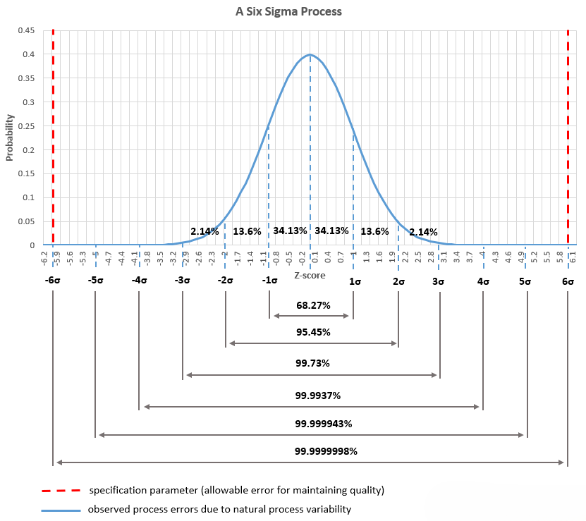
For example, at ~ six sigma, a process operating at this level has a very slim defect rate, even with large production volumes. Note, however, that there are processes out in the real world that do not have this kind of stringent quality control; at least, Three Sigma is usually the target in most industrial settings.
Six Sigma is not simply a quality standard but rather a mechanism of techniques and tools to drive process improvement. This method was initiated at Motorola by engineer Bill Smith and later on commercialized as part of Six Sigma by General Electric (GE) under Jack Welch (the company famously said they saved $1 trillion over ‘the last decade of the 20th century by implementing Six Sigma). According to Smith, to get to a certain sigma, “you’re going to have to reduce the variability in your process, or you can move the specifications over so that a broader and wider range of output is acceptable.
Six Sigma CalculatorManipulation With regard to a process’s sigma level, the six Sigma calculator uses the simple concept that a process should not defect in relation to the number of defects a system produces.
The table illustrates this relationship in terms of defects per million opportunities or defect %, as mentioned below.
| Sigma level | DPMO | Yield | Percent defects |
|---|---|---|---|
| 3 | 2700.0000 | 99.73% | 0.27% |
| 4 | 63.3700 | 99.9937% | 0.0073% |
| 4.645 | 3.4000 | 99.99965% | 0.00045% |
| 5 | 0.5742 | 99.99994258% | 0.00006852% |
| 6 | 0.0020 | 99.9999998% | 0.0000002% |
Rolling throughput yield (unit yield) by sigma level
The 4.64 is what was equated to six sigma in the original work of Smith.
Yield vs. RTY, DPMO vs DPM
The sigma level calculator gives standard yield % (opportunities not failed per total opportunities, and also complimentary to that) plus defects percent, as well, and DPMO (defects per million opportunities) [1]. These are relevant for total process success rate frequency. Nevertheless, if a unit of produce has more than one opportunity, it may be producing a defect; for example each part forms the product, or the service or process itself is made up of several discrete steps and/or has been amended by the sum of multiple measurements than measurements such as DPM metrics defect per million units (defects mille unités options) [2]
Let me show you how they relate and why both are applicable to process control.
If there is only one parameter to tweak for each unit produced, DMP and DMPO are the same, and neither yields RTY. But as soon as parts/products or processes increase — the gap widens exponentially. Smith[1], in his examples, helps show this; a manufacturing process of six sigma quality per part and each part yielding in units with no defects approaches close to 100% (based on 1-10 parts) but falls to 99.9% when parts are 30 and can drop to around the 90.3% mark when the number of steps in the process is 30,000 per with 3.4 DPMO. When the control range is more lax (3-sigma), producing anything in 10 parts would mean over half the units are scraped.
| Process Complexity (parts/unit) | Yield with 3σ* | Yield with 4σ* | Yield with 4.645σ* | Yield with 6σ* |
|---|---|---|---|---|
| 1 | 99.73% | 99.99% | 100.00% | 100.00% |
| 10 | 97.33% | 99.94% | 100.00% | 100.00% |
| 100 | 76.31% | 99.37% | 99.97% | 100.00% |
| 1,000 | 6.70% | 93.860% | 99.66% | 100.00% |
| 10,000 | 0.00% | 53.06% | 96.66% | 100.00% |
| 20,000 | 0.00% | 28.16% | 93.43% | 100.00% |
| 50,000 | 0.00% | 4.21% | 84.37% | 99.99% |
| 100,000 | 0.00% | 0.18% | 71.18% | 99.98% |
Rolling throughput yield (unit yield) by sigma level
* The sigma level refers to the production process of each part. A 4.64σ level is equivalent to what Smith calls 6σ because he includes adjustments for shifts in the average. Here’s how the different sigma levels translate to defects per million opportunities (DPMO): 3σ equals 2700.00 DPMO, 4σ equals 63.37 DPMO, 4.64σ equals 3.40 DPMO, and 6σ equals 0.002 DPMO.
The table above shows the connection between sigma levels for each part and the overall yield in manufacturing units made up of various parts. This same principle applies to all kinds of multi-step processes. You can use the sigma level calculator to perform calculations for any number of parts and sigma levels, as long as each part has the same sigma level. For the nonsigma level, the same parts use the RTY formula.
Sigma Calculator Formulas
Here are some of the most essential formulas in the Sigma calculator with very few explanations.
DPMO formula
Defects per million opportunities The DPMO formula is actually straightforward. First, you take the total number of defects, multiply that by one million, and then divide the result by the total number of opportunities. The total opportunities are determined by multiplying the number of units produced by the number of defect chances per unit. It’s worth mentioning that DPMO is often referred to as PPM (parts per million), a term that originated in the original paper by Bill Smith.

DPMO works better when you examine one process alone. When it comes to more multi-stage processes, DPM (defects per million opportunities) and the rolled throughput yield view the relationship very well.
RTY formula
The equation for rolled throughput yield is given below:

Using the law of error propagation, as described in process control literature since at least 1930, e.g., Shewhart’s classic key work “Economic Control Of Quality Of Manufactured Product”[2], the total error of a series of processes with given yield rates is the individual yield rates multiplied together.
Thus, the defect units rate is 1 – RTY
In the Six Sigma calculator, when you are solving for your sample size, the standard statistical formula relating to confidence intervals is used at the back end.
Sigma shift, long-term vs. short-term sigma?
Some of you may be scratching your heads about why this Six Sigma calculator lacks batch-to-batch variation in its list of inputs. The calculator does not even make use of it implicitly. Why it takes so long
The sigma shift, so-called [1], accounts for lot-to-lot variability of the true mean of the product characteristic (width, length, thickness, diameter, etc.) in manufacturing. Smith cites a mean shift of 1.5σ to be observed in Motorola’s manufacturing processes [6]. Hence, he goes on to tweak the reported sigma levels by moving them all to a perfect 1.5 sigma and thus declaring any method with a sigma level of six.
It appears to me that Smith merely conflated the changes in the mean (which have a fair bit of natural variation) with the fundamental changes of these mean values (fraught with unknown issues). I found no confidence intervals or other uncertainty measures to help us determine the level of confidence in his estimated mean shifts, so it seems we are indeed dealing with this confusion here.
From this, the first misinterpretation seems to have spawned appears to be about short-term vs. long-term sigma:- A 4.64sigma smoothie processing in the short-term would skew to be classified as a long-term 6sigma process because we are allowing for short-term trim of the machinery of 1.5σ. Yet this does not reflect reality. Changes to the mean observed are not actual changes in the mean, and anyway, there would be no downright reason to accept 1.5 sigma as a typical shift since any process will drift from batch to batch and sample to sample. After that, many batches of these effects are canceled out, and that is precisely what the standard deviation of the process (and thus its sigma level) takes into account. In practice, this could mean sampling from multiple lots to weigh them equally or applying a time-decay function if the degradation of manufacturing equipment over time is to be considered.
If underdoing so, it turns out that the mean and sigma of process measurements in batch #1 provide an estimate of three sigma at approx 4.64, then in order to obtain six sigma (and not waving their hand saying they are there when in fact available data implies better than 1,700x fewer defects!) The available data would suggest a much lower number ( one-time defect, hence just one defect), so one cannot just wave a hand and say, “We are Six Sigma now!”S implement, either the math of reducing mean shift has to happen, or we need a method to minimize variability to get the target sigma. If, for example, batch #1 was the first 10 batches of a product and 11 yielded a Sigma estimate of 4.645 (if considered by itself), this may very well mean the machinery needs inspecting and production line repairing instead of assuming things are on the right track. As long as there is natural drift in the mean, the inclusion of this in sigma has to be done.
Ideally, it should be detected before it has much of an impact on quality, a fix is made, and the process is brought under control. Once again, using a sigma shift instead is just lying about how bad the process actually is.
In short, it is more a figment of imagination really of the sigma shift at 1.5, as there is no basis on which this arbitrary number could exist.
Furthermore, any sigma shift applied to calculations on the yield and defect rate of a process amounts to crazy-making of the process’s expected defect rate as well as over-reporting its yield. After all, the entire concept of a “Sigma Score” with no connection to the plain statistical sigma (or even central deviation or anything like it) is nonsense. This is why this sigma-level calculator does not involve a sigma shift~.
This article on sigma shift and reference 3 provide a more elaborate discussion of the 1.5 sigma shift and whether or not any shift makes any control possible for the estimation of long-term or short-term sigma.
Sample size for process control
In process control, you will frequently have to estimate the number of samples that are required to verify that a process is going to be within its specifications. Quality measurements usually entail establishing confidence intervals for the observed sample mean or making comparisons in control charts. Measuring compliance is tiresome, and QM intensive and it can even destroy your element; hence, you need the highest quality control with the minimum sample size possible. And our Sigma calculator comes to your rescue here – choose “sample size” in the interface. For those who want the gory underlying mathematics, continue for more!
In order to figure out the sample size, you have to estimate the standard deviation (σ) in previous samples of the characteristic you want to use as a base for your new sample. The next thing you need to do is to specify a level of probability that the estimation process can use to be really close to estimating the exact value from the characteristic. The same level usually balances the requirement for accuracy with what you are willing to pay (in terms of estimation time) in practice. Also, you have to set the limit of how much you want your interval to be in terms of estimation credibility. This maximum width is essentially half of the standard error (E), often referred to as the margin of error, which is labeled as “maximum error” in the Six Sigma calculator interface.

In order for any meaningful, practical value to be associated with the maximum error being less than the Upper Specification Limit (UCL) minus the lower specification limit(LCL). For example, if the UCL of a rod’s diameter is at 10.2mm and the LCL at 10.0, then the maximum error should never cross 10.2 – 10.0 = 0.2 mm. This is typically a much lower max value to be sure your production specifications are followed.
Suppose past measurement estimates a standard deviation of 0.05 (for 4σ processes, Then the max error can be calculated to be 0.025 (margin of error ± 0.0125). Thus, 62 random samples would need to be measured to ensure that they are within an acceptable tolerance 95% of the time with no more than a 0.025 difference.
Although this is merely a hypothetical illustration, it clarifies how to make use of our free six Sigma calculator properly. You will want to follow the steps in calculating the maximum error (or margin of error = 2*maximum error) that is specific to your scenario.